

The Underrated Science of LLM Samplers
The secret sauce for balancing diversity, quality and precision

Paul: Today’s spotlight: Shmulik Cohen, AI Engineer and Master’s student with a passion for Technology and AI. A tinkerer who must try every new tool by hand and explain to others how to do it. Writing AI Superhero.
This one’s packed, let’s go 👀 ↓
It All Starts With A Single Word
You’ve seen it a hundred times. You ask an LLM the same question twice and get two different, perfectly valid answers. One is a masterpiece, the other is… boring.
This “creativity” might seem like random luck, but the truth is, it’s one of the most important (and controllable) parts of an LLM. The magic isn’t just in the model’s massive size, it’s in a small, powerful component called the Sampler.
Mastering samplers lets you choose between predictable, consistent text and exactly the novel, creative output you desire in other cases. To understand what a sampler does, we first need a super-quick look at how an LLM works.
Softmax
How An LLM Writes: From “Once Upon a Time” To… What?
At its core, an LLM is a giant probability machine. When you give it a prompt like “Once upon a time, there,” it doesn’t “think” of what to say next in the way a human does.
Instead, it performs two simple steps:
It calculates a score (called a logit) for every single possible word (or “token”) in its vocabulary (often 50,000+ words) that could come next.
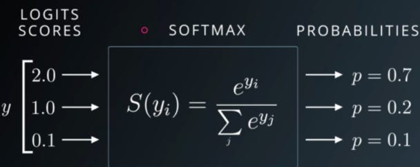
It uses a function called Softmax to convert that list of raw scores into a list of probabilities that all add up to 100%.
For example, after “Once upon a time, there”:
“was”: (score: 10.2) -> Softmax -> 70%
“lived”: (score: 8.5) -> Softmax -> 15%
“in”: (score: 7.1) -> Softmax -> 5%
“dwelt”: (score: 6.0) -> Softmax -> 1.5%
“galloped”: (score: 2.0) -> Softmax -> 0.1%
“aardvark”: (score: 0.01) -> Softmax -> 0.00001%
…all other 49,995 words… : < 8.4%
The Math Behind Softmax
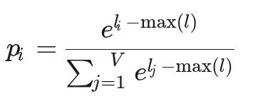
The Softmax function takes the list of all logits and turns each one into a probability by taking its exponential and dividing it by the sum of all the exponentials.
This sounds complex, but it’s just a way to ensure two things:
Words with higher scores get a much higher probability.
All the probabilities add up to 1 (or 100%).
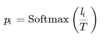
The formula for a single word’s probability (p_i) from a list of vocabulary words (V) is (for implementation details, check out Appendix A):
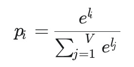
And in a simplified diagram:
This final probability list is the LLM’s “best guess.” Now comes the most important question: Which word do we actually pick?
What Is An LLM Sampler?
This is where the sampler comes in. An LLM sampler is the algorithm that takes this list of probabilities and picks one (and only one) word.
How it picks that word has a massive impact on the output, forcing a constant balance between two extremes:
The Sampler’s Trade-off: Too Predictable ← — — — — — — — -> Too Chaotic
Let’s look at why navigating this trade-off is essential.
Extreme #1: The “Predictable” Pitfall (Greedy Sampling)
The simplest strategy is called Greedy Sampling (or Greedy Decoding). It’s not really “sampling” at all. It just looks at the list and always picks the single word with the highest probability.
In our example, it would pick “was” (70%) every single time.
Why it’s a problem: It’s 100% predictable and deterministic. Imagine asking it to write stories about children — every kid would end up with the most common name (like “John” or “Mary”), like the most common game (like “tag”), and prefer the most common color (“red” or “blue”).
If you use greedy sampling, your LLM becomes a repetitive parrot, writing the exact same, most probable text every single time for the same prompt. There is zero creativity or variation.
Extreme #2: The “Chaotic” Pitfall (Unfiltered Sampling)
What about the other extreme? What if we sample from the entire 50,000-word list, respecting all probabilities?
Why it’s a problem: This method has two major flaws:
First, the risk compounds. A 0.00001% chance of picking “aardvark” seems tiny, but you are rolling those dice for every single word you generate. When writing a long text, this tiny chance of disaster compounds. Over a full paragraph, the odds of at least one catastrophic, out-of-place word appearing become unacceptably high. The model will say, “Once upon a time, there aardvark…” and the entire generation is derailed.
Second, it gives you zero control. This method is stuck on one setting: “chaotic.” Greedy sampling is stuck on another: “predictable.” You have no “knob” to dial in the behavior you actually want, whether it’s precise for a technical summary or creative for a story.
The Sampler’s Toolkit: Finding The Sweet Spot
So, the goal of a good sampler is to find that sweet spot: to be creative, but not chaotic. We need methods that filter out the “noise” while still considering reasonable creative options beyond just the single best word. Most importantly, we need a “knob” that lets us choose between precision and creativity depending on the task, without hurting the quality.
This is where the different sampling algorithms come into play. To see exactly how they work, I’ll be using a visualization tool originally created by Romain D, which I modified (more on that at the end!). The code examples use llm-samplers, a small library by Ian Timmis, which makes it easy to plug and play with different methods.
llm-samplers SetupFirst, let’s get the library installed:
pip install llm-samplersNow, let’s write a simple script to generate text. We’ll use a small, fast model (SmolLM-135M) so you can easily run this yourself.
For our first test, we’ll use TemperatureSampler(temperature=1.0). This is a good “neutral” baseline—it doesn’t sharpen or flatten the probabilities, just samples from them as the model intended.
And start to use it with this simple template
from llm_samplers import TemperatureSampler
from transformers import AutoModelForCausalLM, AutoTokenizer

# Load model and tokenizer
model = AutoModelForCausalLM.from_pretrained(”HuggingFaceTB/SmolLM-135M”)
tokenizer = AutoTokenizer.from_pretrained(”HuggingFaceTB/SmolLM-135M”)

# Initialize a naive sampler
sampler = TemperatureSampler(temperature=1.0)

# Generate text with the sampler
input_text = “Once upon a time”
input_ids = tokenizer.encode(input_text, return_tensors=”pt”)
output_ids = sampler.sample(model, input_ids, max_length=30)
generated_text = tokenizer.decode(output_ids[0])
In one of my runs, I got this. It’s coherent, but you can see it starting to drift a little, a perfect example of that T=1.0 randomness.
“Once upon a time, a curious girl named Maya wore glasses and had guests for breakfast every day. Maya loved the way her mom looked at her and explained the principles of”
Visualizing The Probabilities
That text output is helpful, but to really understand what’s happening, we need to see the probabilities.
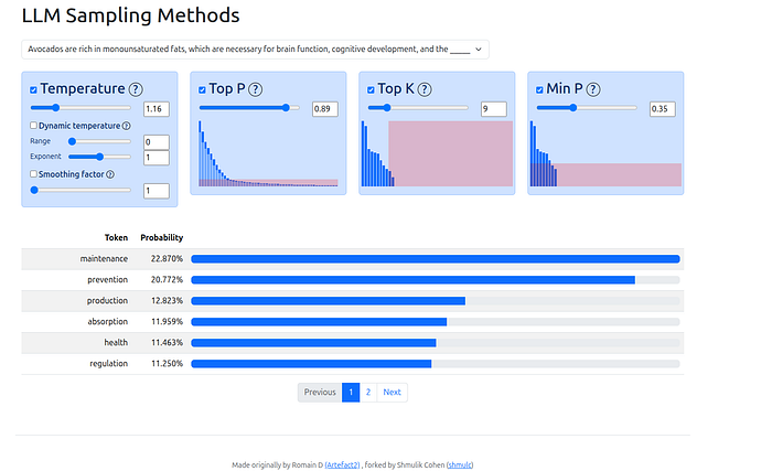
This is where the LLM Sampling Visualization tool comes in. It runs a prompt and shows us the exact probability list the model generates for the very next word. This lets us see precisely how each sampler modifies that list before making a choice
You can follow along here: https://anuk909.github.io/llm-sampling/web/
For our examples, we’ll use the prompt:
”No, Johnny, Steve didn’t jump off a bridge. That was just a figure of speech. I’m glad you’re…”
Here is the raw, unfiltered probability list (the result of Softmax) for the next word. This is our “baseline” before any sampling is applied:
Now, let’s see what happens when we start turning the “knobs.”
Sampling Methods
Temperature 🌡️ (The “Spice” Knob)
What it is: Temperature is usually the first adjustment made to the LLM’s raw output probabilities. Unlike the methods below, it doesn’t remove any words from consideration. Instead, it adjusts the “sharpness” or “flatness” of the entire probability distribution before any filtering happens. Think of it as the foundational level for the text generation: a little makes it flavorful, too much makes it incoherent.
Low Temp (e.g., 0.7): Makes high-probability words even more likely and low-probability words even less likely. This “sharpens” the distribution, making it safer, more predictable, and more like greedy sampling.
High Temp (e.g., 3.0): Makes all words more equal. It “flattens” the distribution, giving “riskier,” less likely words a better chance. This makes the model more random and “creative.”
The Math: It’s a simple idea. Before the softmax, it divides the logits by the temperature value (T).
Visualization: Here’s what our example looks like with a different temperatures, you can see how the distribution with low temperature is sharper and with high temperature is much more flat.
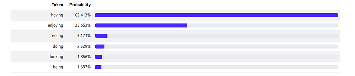
Temperature = 0.7
Temperature = 3.0
How to Use It (llm_samplers):
from llm_samplers import TemperatureSampler

# More deterministic (picks high-probability tokens)
sampler = TemperatureSampler(temperature=0.7)

# More random (flatter distribution)
sampler = TemperatureSampler(temperature=3.0)
Low Temp: Once upon a time, there was a group of friends who loved to play together. They would gather around a big bonfire in the forest, sharing stories and laughter while
High Temp: Once upon a time Feet Allen Lau Celsius purse publishes button trajectory Lalono greetings Relationship talked chairman Certainly washing strategicademayama Library Perc poisons polymatos SNPs[ url multiplex Pop titanium
The results speak for themselves. High temperature alone can quickly lead to nonsense. Now let’s look at methods designed to filter these probabilities.
Top-K (K)📋 (The “Fixed Menu”)
What it is: This sampler is very simple. It just cuts off the list after the K most probable words and samples only from that group.
The Logic: It says, “I don’t care about the probabilities. Just give me the Top 50 words, throw the other 49,950 in the trash, and I’ll pick from that Top 50 list.”
The Problem: It’s not adaptive. Sometimes the real choice is between 3 words. Sometimes it’s between 200. A fixed K=50 might be too small in one case (cutting off good options) and way too large in another (letting in “aardvarks”).
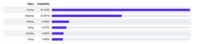
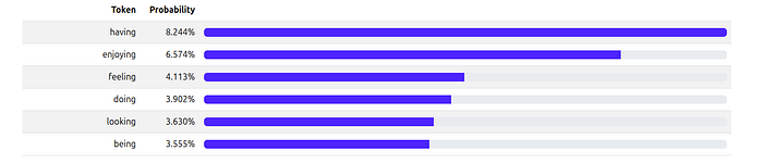
Visualization: Here, we set K=3. The sampler “truncates” the list, keeping only the top 3 words (“having,” “enjoying,” “feeling”) and throwing everything else away. It then re-calculates the probabilities among just those three.
How to Use It (llm_samplers):
from llm_samplers import TopKSampler

# Consider only the best token (greedy)
sampler_top_k = TopKSampler(k=1)

# Consider only the top 10 tokens
sampler_top_k = TopKSampler(k=10)
Top 1: Once upon a time, there was a curious little girl named Lily. She loved exploring her backyard and playing with her friends. One day, she noticed that her favorite toy
Top 10: Once upon a time, there was a young boy named Timmy who had just started kindergarten. At the time, Timmy didn’t know much about the world, but he loved
Top-P / Nucleus Sampling (p) 🎯 (The “Smart Menu”)
What it is: This is a much smarter, adaptive version of Top-K. Instead of picking a fixed number of words, it selects the smallest set of tokens whose cumulative probability exceeds a threshold ‘p’
The Logic: It sorts the words from most to least likely and adds them to a “nucleus” list, one by one, until their combined probability reaches P (e.g., 95% or 0.95).
“ok” (35%) -> Add to list. (Total: 35%)
“not” (18%) -> Add to list. (Total: 53%)
“worried” (10%) -> Add to list. (Total: 63%)
… (keeps adding) …
“glad” (2%) -> Add to list. (Total: 96%) -> STOP.
The sampler will now only pick from the 10–15 words that made it into that 95% “nucleus.”
The method is adaptive!
If the model is “certain” (e.g., one word has a 95% chance), the list will only have 1 word.
If the model is “uncertain” (e.g., the top 100 words add up to 90%), the list will have 100 words.
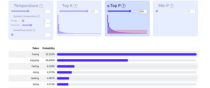
Visualization: Here, with P=0.8, the sampler includes the top 6 tokens until their combined probability hits 80% and re-calculates the probabilities among these.
How to Use It (llm_samplers):
from llm_samplers import TopPSampler

# Consider tokens that make up 50% of the probability mass
sampler_top_p = TopPSampler(p=0.50)

# Consider tokens that make up 90% of the probability mass
sampler_top_p = TopPSampler(p=0.90)
Top 50%: Once upon a time, there was a group of friends who loved to play together. They would gather around to watch their favorite show, which was called “Dance and
Top 90%: Once upon a time, there was a man named Manel who lived in a faraway land called North Africa. When he grew up, he decided to learn more about different
Min-P Sampling 🚀 (The New Challenger)
What it is: This sampler is a brilliant new approach that dynamically adjusts the sampling pool based on the probability of the most likely token.
The Logic: Top-P has a subtle flaw. If the list is: “was” (50%), “lived” (45%), “dwelt” (5%), Top-P (p=0.9) will only pick [”was”], cutting off “lived” even though it was a great alternative.
Min-P solves this. It looks at the #1 top word (let’s say it has a 30% chance) and multiplies that by a value P (e.g., 0.1).
30% (prob of #1 word) * 0.1 (Min-P value) = 3%
Now, the sampler will discard any word with a probability less than 3%.
This is brilliant because:
It solves the “long tail” problem by setting a hard minimum, kicking out the 0.0001% “aardvarks.”
It solves the Top-P problem by keeping high-quality “runner-up” words (like “lived” at 45%) that might have been unfairly cut.
It’s fully adaptive: if the model is certain (top word is 90%), the cutoff is high (9%). If the model is uncertain (top word is 10%), the cutoff is low (1%), letting more creative options in.
A Nod to the Source: This method was introduced in the paper “Turning Up the Heat: Min-p Sampling for Creative and Coherent LLM Outputs”.
One of its biggest advantages is that it can work very well even with high temperatures, allowing for creativity while maintaining coherence.
Their experiments showed Min-P significantly outperforming Top-P on benchmarks like GSM8K and creative writing, particularly when using temperatures above 1.0. And even more impressive: the human evaluations showed a clear preference for Min-P outputs in terms of both quality and diversity, which means that it’s not only better at the benchmarks, people liked it more too!
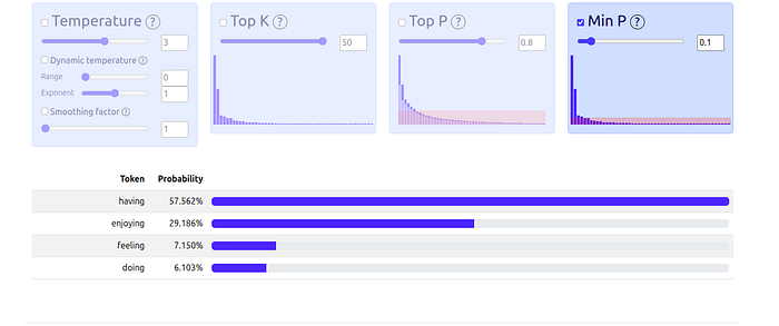
Visualization: With Min-P=0.1, the top token “having” is at ~43%. The cutoff becomes 4.3%. The sampler keeps every token above 4.3%, which in this case is a small, high-quality list of 4 tokens.
How to Use It (llm_samplers):
from llm_samplers import MinPSampler

# Use min-p sampling with a threshold of 0.1
# This means a token must be at least 10% as probable as the top token
sampler_min_p = MinPSampler(min_p=0.1)
min_p=0.1: Once upon a time, there was a curious little girl named Maya who loved learning about the world around her. She spent hours reading books, watching documentaries, and even participating
Combining Samplers And Other Methods
You don’t have to pick just one! In fact, the most common way to use samplers is to combine them. A very popular combination is using Temperature (to sharpen or flatten the list) and then using a truncation method like Top-P or Min-P (to cut off the long tail). This gives you multiple knobs to tune for the perfect balance. The interactive site allows you to play with the different methods, and even their order ,to see for yourself how these combinations change the results.
And the rabbit hole goes deeper. The llm-samplers library includes even more creative methods. For example, XTC (Exclude Top Choices) Sampling is designed to enhance creativity by nudging the model away from its most predictable choices, or Beam Search, which searches for the Top-K most promising sequences (entire phrases), not just single tokens.
I haven’t touched on these in detail here, but it shows how much active research is going into this one “simple” step.
My “Aha!” Moment With Samplers
I was inspired to dive deep into this topic after watching an excellent lecture at an AI Tinkerers Meetup by Ravid Shwartz-Ziv, one of the authors of the Min-P paper. His talk clarified just how much control we have over LLM output.

I already knew about sampling and Temperature, but the lecture showed me how a smart sampler is the real key to balancing coherence and creativity. It’s not just about one setting, it’s about a whole toolkit.
A Note On The Tools: My “Rabbit Hole” Project
While working on this post, I hit a roadblock: How do you visually show the difference between these samplers in action? Static pictures are okay, but I wanted an interactive tool.
I searched for an existing solution and found a repository that was almost perfect… but it was old, broken, and built on PHP. 🤦♂️
So, I fell down a rabbit hole for a few hours and ended up rewriting the project from scratch to be modern, aesthetic, and reproducible. The result is the visualization tool used throughout this post:
Live Demo: An interactive site where you can see exactly how these samplers filter a real LLM’s output. https://anuk909.github.io/llm-sampling/web/
GitHub Code: The source code for the visualization tool itself. https://github.com/anuk909/llm-sampling
It was a fun detour, and hopefully, the tool helps make these concepts clearer!
Final Thoughts: Choosing Your Sampler
Samplers are the unsung heroes of LLM generation. They are the crucial “knobs” that let you dial in the balance between creativity and coherence, tuning your model from a repetitive parrot into a dynamic creative partner, or vice-versa.
As we’ve seen, different samplers, like Temperature, Top-K, Top-P, and the newer Min-P, operate on different principles and produce distinct results. There’s no single “best” sampler, the ideal choice depends entirely on your specific task. Are you aiming for factual accuracy, freewheeling creativity, or something in between? Understanding these methods gives you the control to achieve your goal.
This is also an active area of research, with new techniques and refinements emerging regularly. Staying updated on the latest methods and best practices can help you get the most out of LLMs.
While we used the llm-samplers library for demonstrations in this post, keep in mind that these core sampling methods (Temperature, Top-P, Top-K, Min-P) are fundamental concepts. You’ll find them available as parameters in most major LLM libraries (like VLLM and transformers) and APIs (like those from OpenAI, Anthropic, Google, etc.), giving you the power to control text generation wherever you use LLMs.
The next time you’re working with an LLM, pay attention to the sampler, it might be the key to unlocking the output you’re looking for.
Appendix A: Numerical Stability In Softmax
Calculating e^x directly is risky. A large logit can cause an “overflow” (a number too big to store), while all-negative logits can cause an “underflow” (leading to a 0/0 error).
To fix this, libraries use a clever trick: they subtract the largest logit from all other logits before exponentiating, based on the identity
softmax(x) = softmax(x + c).
This is mathematically identical and guarantees a stable calculation. The max exponent becomes 0, so the largest value is e⁰ = 1, preventing overflow. The sum in the denominator also now includes at least one 1 term, preventing a vanishing denominator and a division-by-zero error.
Till next time.
Shmulik Cohen | LinkedIn | AI Superhero Substack
What’s your opinion? Do you agree, disagree, or is there something I missed?
Enjoyed the article? The most sincere compliment is to share our work.
Whenever you’re ready, here is how I can help you
Go from agent user to agent builder. Master the foundations of AI agents and turn fragile demo code into reliable, production-ready systems with my course, Agent Engineering: Building Multi-Agent Systems (made with Towards AI).
35 lessons. Pure foundations from scratch. 4 mini-projects. 2 production systems. A certificate and direct access to me & industry experts in our Discord.
Built for software and data professionals transitioning into AI engineering. Rated 5/5 with 300+ students. The first 7 lessons are free:
Not ready to commit? Start with our free Agent AI Engineering Guide, a 6-day email course on the mistakes that silently break AI agents in production.
Images
If not otherwise stated, all images are created by the author.
 | A guest post by
|
Thank you, Shmulik, for contributing this amazing piece!
🎩💙🍷🖖